The Subject of Probability

Probability is the basis for statistics and an intricate tool used for dealing with what we call non-deterministic events; that is, we do not know the outcome of an event before it occurs. Most of mathematics deals with deterministic events, e.g. “If I have 5 coins and you take 1 away, I have 4 coins left.” Probability does not work the same way since I can flip a coin several times and each flip can come out differently. It is often described as “being up to chance” what the outcome will be even though chance is not an actor that can be responsible for anything. What is responsible for different results? We do not know. In events where not everything is known, we rely on probability to help us understand what can happen. Because of this, it is essential to be certain of one’s interpretation of probability, especially when looking to make decisions.

We all think that we understand probability, but as mentioned before probability is an intricate tool. Take special care with the definitions provided in this chapter. Probability is not an intuitive subject. Random improbable events happen, and yet we are surprised when they happen to us. The exclamation “Impossible! There was only a 1% chance of that happening!” contradicts itself. The one-percent chance is a very real chance. In our minds, we have some belief about how probable an event is to happen and often we say a 1% chance is not enough to consider a valid possibility and we discard it. Perhaps for small stakes this is acceptable, but in other cases the 1% chance of a large loss may need to be considered. In fact, if the experiment where the undesirable outcome can happen is performed 1000 times, it would be more surprising not to see this outcome at least once.

This chapter explains how use probability as a tool instead of as a reason to dismiss the improbable.

What is a Probability?

First, let us define a probability (or a chance as is often used) as “the expected frequency with which a certain outcome is observed when an experiment is repeated indefinitely.” This tells us a couple things about a probability. Its value is always between 0 and 1, and its “true” value can never be observed since we cannot infinitely flip a coin or repeat any other sort of experiment. However, because it is an expected frequency, we do not need to know the “true” value of a probability to make use of it.

Another detail we must specify is whether this experiment has been performed already or not. In this course, we will approach problem from a subjectivist’s perspective where anything unknown can be assigned a probability. This is opposed to a frequentist’s perspective which is only concerned with the true state of the world. Say a teacher tosses a coin, catches it, and asks a student the probability of it being heads. Most people would say 50 percent without even thinking. They are saying that they expect the coin to be heads just as much as they expect it to be tails. A frequentist would say, “You have already tossed the coin. Probability is not appropriate in this situation.” This course is not designed for that inflexible kind of thinking. Instead, we will use the subjectivist perspective since that is more similar to the way we already think of probability.

Probability Terms

TODO: I need to find a way to use these in a narrative to illustrate them. * sample space - the set of all possible outcomes and events from an experiment; also, the set of values (or domain) that a random variable can take on * experiment - a situation with one or more outcomes; remember, in our interpretations the experiment can already have run to completion without us having observed an outcome * random variable (rv) - a component in an experiment that takes on a value * outcome - the state of our random variable at the end of an experiment, whether observed or not * state - a deterministic value for a variable * event - a set of outcomes for an experiment; e.g. \(A\) can be defined as rolling a pair of dice and obtaining an even number

Random Variables

Random variables are one of the building blocks of probability. Instead of blaming chance, we define a random variable which encapsulates all of the unknowns influencing a particular value in our experiment. The value of this random variable will change from experiment to experiment (if we have multiple experiments).

Mathematically, rvs have certain properties.

1. rvs can either be discrete or continuous. Discrete means they can only take on certain values, often nonnegative whole numbers. Continuous means they can take on any value within a certain range such as \((-\infty, \infty)\) or \([0, \infty)\) or \([0,1]\).

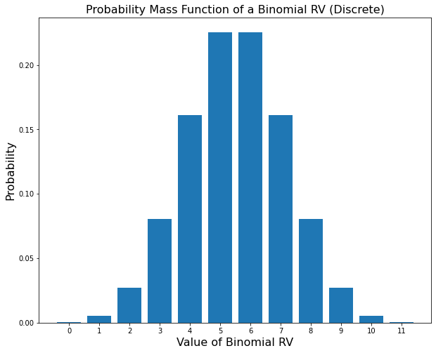
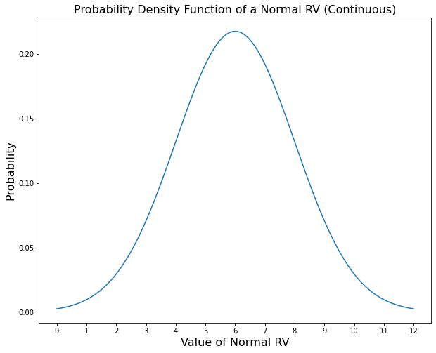
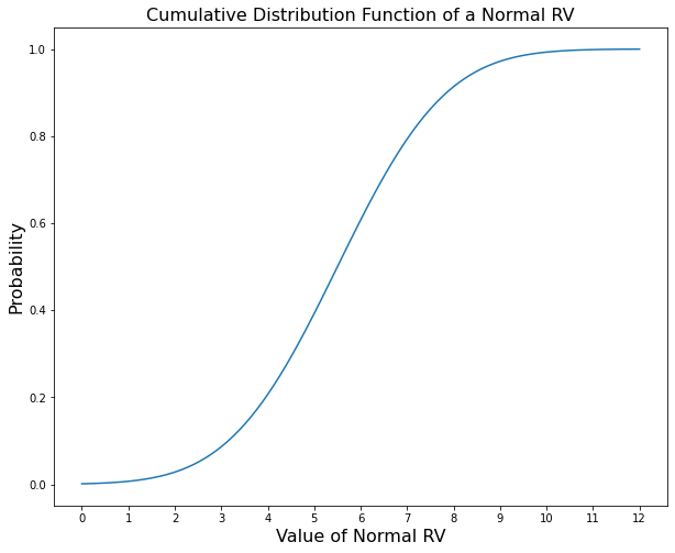
2. Discrete rvs have a pmf or probability mass function which gives the relative probability/frequency of them taking on a value and it is written as \(P(X=k) = f_X(k)\). Continuous rvs had a pdf or probability density function which also gives the relative probability/frequency of them taking on a specific value. It is written as \(P(x<X\leq dx) = f_X(x)\). Continuous rvs also have a cdf or cumulative distribution function. This gives the probability of \(X\) being less than or equal to a certain value. It is written as \(P(X \leq x) = F_X(x)\). Below are some examples of these functions

import numpy as np
from scipy.stats import binom, norm
import matplotlib.pyplot as plt

plt.figure(figsize=(10,8))
plt.bar(np.arange(0,12), binom.pmf(np.arange(0,12), 11, .5))
plt.title("Probability Mass Function of a Binomial RV (Discrete)", fontsize=16)
plt.ylabel("Probability", fontsize=16)
plt.xlabel("Value of Binomial RV", fontsize=16)
plt.xticks(np.arange(0,12))
plt.show()

plt.figure(figsize=(10,8))
plt.plot(np.linspace(0.,12,100), norm.pdf(np.linspace(0.,11.,100), 5.5, 5.5/3.))
plt.title("Probability Density Function of a Normal RV (Continuous)", fontsize=16)
plt.ylabel("Probability", fontsize=16)
plt.xlabel("Value of Normal RV", fontsize=16)
plt.xticks(np.arange(0,13))
plt.show()

plt.figure(figsize=(10,8))
plt.plot(np.linspace(0.,12.,100), norm.cdf(np.linspace(0.,12.,100), 5.5, 5.5/3.))
plt.title("Cumulative Distribution Function of a Normal RV", fontsize=16)
plt.ylabel("Probability", fontsize=16)
plt.xlabel("Value of Normal RV", fontsize=16)
plt.xticks(np.arange(0,13))
plt.show()

3. Discrete rvs can have distributions (pmf’s) with irregular intervals between possible values, and continuous rvs can have distributions (pdf’s) that are not differentiable. Essentially, whatever distribution you can conceive, a rv can have. This allows rv’s to represent something as flexible as human beliefs.

4. There are many predefined discrete and continuous probability distrbutions. Above are shown examples of binomial and gaussian/normal distributions. Often, probability distributions are suited to specific kinds of events. For instance, a binomial distribution represents the probability of observing a certain number of successes \(k\) in an experiment with \(n\) trials where each trial has a probability of success \(p\). Thus if \(X\) is a rv that has a binomial distribution, then the probability that \(X\) is equal to any value \(k\) can be written as pmf \(f_X(k; n, p) = {n \choose k} \cdot k^p \cdot (n-k)^{1-p}\).

   The normal distribution is less interpretable but is often used to represent a variable that has an equal chance of being above or below its expected value by a certain distance. Just as the pmf of a binomial distribution is parametrized by \(n\) and \(p\), a normal distribution is parametrized by \(\mu\) and \(\sigma\) where \(\mu\) is the expected value of the variable and \(\sigma\) is proportional to the distance observed above or below the mean. A rv \(Y\) that is normally distributed has a pdf \(f_Y(y; \mu, \sigma^2) = \frac{1}{\sigma\sqrt{2\pi}} \cdot \exp\left({\frac{(y-\mu)^2}{2\sigma^2}}\right)\)

   rvs with a parametrized distribution like this are often defined in the following manner. A binomial rv \(X\) is defined by \(X \sim \text{Binom}(n, p)\) and a normal rv \(Y\) is defined by \(Y \sim N(\mu, \sigma^2)\). The two variables shown are \(X \sim \text{Binom}(11,.5)\) and \(Y \sim N\left(5.5, \left(\frac{5.5}{3}\right)^2\right)\). And remember these are just two distributions out of many.

5. Probability distributions can also be described in other ways. For example, numeric random variables all have expected values and variances, written as \(E(X)\) and \(\text{Var}(X)\). The expected value can also be called the mean, or the average of all the values we would see if we conducted a large number of experiments. The variance is representative of how spread out the values between experiments should be. The square root of the variance is what we call standard deviation and is another measure for how much a random variable can vary. There are also other metrics such as skewness and kurtosis which we will not touch on in this course as they have little relevance, nor will we discuss how to calculate any values other than expected value. It suffices to know how to find a mean and that as variance (or standard deviation) increases, so will the distance between observations.

Joint, Marginal, and Conditional Probability

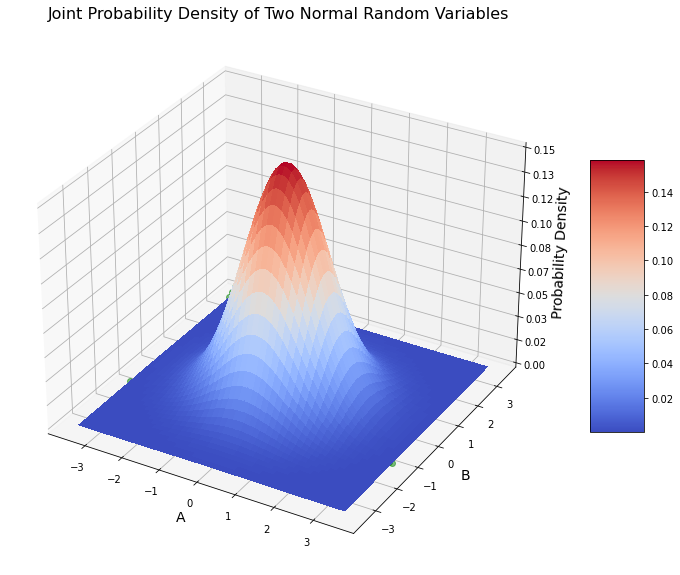
The last essential concept we need to know about probability is how random variables interact with each other. This where we define joint, marginal, and conditional probability. Up until now, we have only considered using a single random variable at a time. Each random variable has a 1-dimensional domain or sample space. Both \(X\) and \(Y\) previously have 1 value they can take on at a time. For \(X\) the domain is \([0,1,2,3,4,5,6,7,8,9,10,11]\). For \(Y\) it is all real numbers \((-\infty, \infty)\). Because they are 1-dimensional we can graph them on the x-axis and the pmf, pdf, or cdf on the y-axis as shown.

If we like, we can also visualize the probability of two variables taking on a specific set of values. Let’s say we have two independent random variables \(A\) and \(B\) which both have a standard normal distribution (that is, \(N(0,1)\)). Their probability density together at any point in 2-dimensional space would look like this:

from matplotlib import cm
from matplotlib.ticker import LinearLocator

fig, ax = plt.subplots(subplot_kw={"projection": "3d"}, figsize=(14,10))

# Make data.
x = np.linspace(-3.5, 3.5, 100)
y = np.linspace(-3.5, 3.5, 100)
X, Y = np.meshgrid(x, y)

line = norm.pdf(x) * norm.pdf(-.9)

Z = norm.pdf(X) * norm.pdf(Y)

# Plot the surface.
surf = ax.plot_surface(X, Y, Z, cmap=cm.coolwarm,
                       linewidth=0, antialiased=False)
ax.plot(x, np.full(100,-1.3), line, 'go', alpha=.5)

# Customize the z axis.
ax.set_zlim(0, .15)
ax.zaxis.set_major_locator(LinearLocator(10))
# A StrMethodFormatter is used automatically
ax.zaxis.set_major_formatter('{x:.02f}')

# Add a color bar which maps values to colors.
fig.colorbar(surf, shrink=0.5, aspect=5)

ax.set_xlabel('A', fontsize=14)
ax.set_ylabel('B', fontsize=14)
ax.set_zlabel('Probability Density', fontsize=14)
plt.title('Joint Probability Density of Two Normal Random Variables', fontsize=16)

plt.show()

Independent Variables

Bayes’ Rule

• Joint probability (marginal probability, conditional probability)

• Independent variables

• Properties of pmf’s and pdf’s

  • Expected value/mean

  • Variance/standard deviation

• Different probability distributions

• Bayes’ Rule